Creating a Voronoi Diagram of the Toronto Subway System
- Rohan Dawar
- Aug 17, 2021
- 5 min read
Updated: Jan 3, 2022
A Voronoi Diagram is a plane consisting of points and polygons. The polygons, or Voronoi Cells surrounding each point represent the area closer to that point than another point on the plane. Essentially, all area within a polygon X is more proximal in Eucliadian distance to point X than to any other point. Like this:

These polygons are derived from the very cool "Voronoi expansion" as seen below:

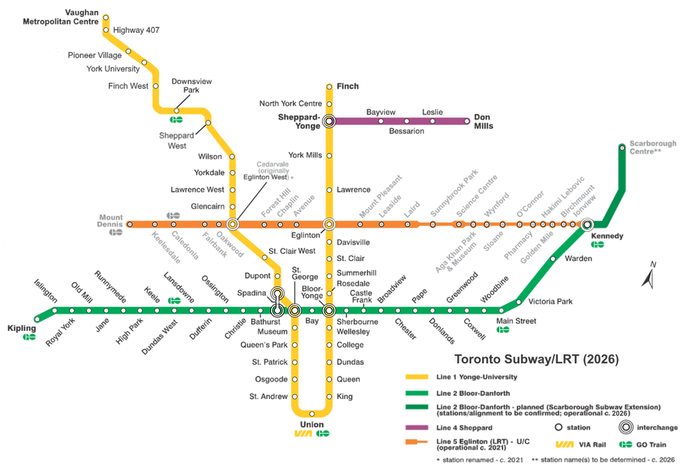
In this project, I will be creating a Voronoi map of Toronto's Subway System (TTC) with points corresponding to stations. The resulting map will act as a reference for which station is closest to any area in the city. It will also show us relative station "catchments" and polygon areas, which could be useful for commuters, newcomers to the city, and informing future transit expansions.
I will be using geovoronoi to create the voronoi polygons and folium & geopandas for mapping. I will also be using pandas for dataframes and BeautifulSoup for webscraping. Let's go ahead and install + import these packages:
Outline:
Dependencies:
!pip install -U geovoronoi[plotting]If running in a Jupyter Notebook, you may have to restart your runtime after running the above code cell for it to properly install.
!pip install geopandas
!pip install descartes
import pandas as pd
import numpy as np
import requests
from bs4 import BeautifulSoup
import matplotlib.pyplot as plt
from shapely.geometry import Point
import geopandas as gpd
import folium
from geovoronoi.plotting import subplot_for_map, plot_voronoi_polys_with_points_in_area
from geovoronoi import voronoi_regions_from_coords, points_to_coordsWikipedia Page to Pandas Dataframe:
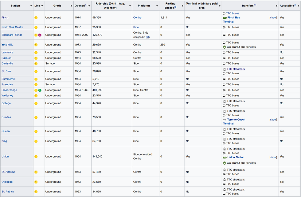
url = 'https://en.wikipedia.org/wiki/List_of_Toronto_subway_stations'Table 1 in the wikipedia page contains the list of all existing stations. We will store this as a dataframe called existing:
existing = pd.read_html(url)[1]
We can see that the table does not contain coordinates, so we must create a small web-scraper using beautifulsoup to parse coordinates from each station's individual wikipedia page.
Parsing Wiki Links for Each Station:
First we can grab the table containing the existing stations:
response = requests.get(url)
soup = BeautifulSoup(response.text, 'html.parser')
table = soup.find_all('table')[1]
Next a short loop grabbing the links from the station name column values:
links = []
for tr in table.findAll("tr"):
  trs = tr.findAll("th", scope='row')
  for each in trs:
    try:
      link = each.find('a')['href']
      links.append(link)
    except:
      pass
Finally, we can add these links in a new column on the existing dataframe:
existing['Link'] = linksGetting Lat/Long Coordinates for Each Station:
base_url = 'https://en.wikipedia.org'I've written a short function that scrapes page for its main coordinates in the "geo" class:
def get_coords(link):
  r = requests.get(base_url + link)
  soup = BeautifulSoup(r.text, 'html.parser')
  coordstring = soup.find(class_="geo").text.strip()
  tuplestring = tuple(map(float, coordstring.split(';')))
  return (tuplestring[1], tuplestring[0])
Applying function to dataframe's 'Link' column:
existing['coords'] = existing['Link'].apply(get_coords)Getting & Assigning Colours:
There is a useful wikipedia template containing the official hexadecimal TTC colours we can scrape into a python dict:
 COLurl = 'https://en.wikipedia.org/wiki/Template:TTC_color'
 colorHash = pd.read_html(COLurl)[1]
 websafeCOLS = {colorHash['Color.2'][i]:
 colorHash['Web-safeHexadecimal.1'][i] for i in colorHash}
 colorHash = colorHash[1:6]
 colorHash = colorHash['Color.2'].to_dict()
Scraper for line number:
response = requests.get(url)
soup = BeautifulSoup(response.text, 'html.parser')
table = soup.find_all('table')[1]

lines = []
for tr in table.findAll("tr"):
  trs = tr.findAll("td")
 for each in trs:
     try:
        link = each.find('a')['href']
        if link.split('/wiki/')[1][0:4] == 'Line':
            lines.append(link)
     except:
         pass

existing['LineLink'] = lines[1:]
Next we can extract the line number from the URL link:
 def extractLineNO(LineLink):
     return int(LineLink.split('/wiki/Line_')[1][0])

 existing['LineNO'] = existing['LineLink'].apply(extractLineNO)
Shapefile & Geopandas Geodataframe:
I will be using a pre-downloaded shapefile for all of Canada but this step could be a web-scraper as well.
Since we will be plotting latitude and longitude, we need to convert the coordinate reference system (CRS) to 'WGS 84', the standard coordinate for ellipsoid latitude and longitude:
canada = gpd.read_file('/content/lpr_000b16a_e.shp')
canada = canada.to_crs('WGS84')
Next we can narrow down the geometry to just the province of Ontario, where Toronto is located. I won't be using a shapefile of the City of Toronto because the TTC subway system extends beyond the boundaries of the city proper.
ontario = canada[canada['PRNAME'] == 'Ontario']
ontariogeo = ontario.iloc[0]['geometry']
Let's plot our coordinates:
fig, ax = plt.subplots(figsize=(12,12))
ontario.plot(ax=ax)
ax.set_xlim(-79.6,-79.2)
ax.set_ylim(43.6,43.8)

for i in range(len(existing)):
  d = existing.iloc[i]
  cds = d['coords']
  ax.plot(cds[0], cds[1],  marker='o', markersize=4, color='red', markeredgecolor='black', alpha=1, zorder=10)
Validity Checks:
Just as a precaution, we will double check that our geometry is valid and our coordinates all intersect with our geometry:
Valid geometry check:
if not ontariogeo.is_valid or ontariogeo.is_empty:
 print('Invalid Geometry')
else:
 print('Geometry Valid')
Depending on the geometry and voronoi function, some cases will require a polygon instead of a MulitPolygon object, if this were the case, we could select the main polygon with the following code:
biggestpoly = max(ontariogeo, key=lambda a: a.area)Regardless of if our geometry is a polygon or MultiPolygon object, we should check if all our coordinates intersect with it:
for i in existing:
  cds = i['coords']
  name = i['Station']
  p = Point(cds[1], cds[0])
  if not ontariogeo.contains(p):
     print(f'{name} ||| OUTSIDE BOUNDARY')
Creating Voronoi Polygons:
In order to create Voronoi Polygons, our coordinates must be in a numpy array of lists:
arcords = np.array(list(map(list, existing['coords'].tolist())))Voronoi function:
region_polys, region_pts = voronoi_regions_from_coords(arcords,ontariogeo)Plotting in Matplotlib:
fig, ax = plt.subplots(figsize=(12,12))
plot_voronoi_polys_with_points_in_area(ax, ontariogeo, region_polys, arcords, region_pts)
ax.set_xlim(-79.6,-79.2)
ax.set_ylim(43.6,43.8)
Mapping in Folium:
We could get the mean center of our coordinates for the starting map location.
I'll be using CartoDB positron tiles:
m = folium.Map(location=[43.65, -79.4], zoom_start=13, tiles='CartoDB positron')Polygons:
for count, r in enumerate(region_polys.values()):
  dfindex = region_pts[count][0]
  d = existing.loc[dfindex]
  col = d['COL']
  websafecol = '#' + websafeCOLS[col]
  name = d['Station']
  opened = d['Opened[6]']
  rdshp = d['Ridership (2018[7] Avg. Weekday)']

  popup = f'{name} Station\nOpened: {opened}\nRidership (2018, weekday): {rdshp}'

  geo_j = folium.GeoJson(data=r, style_function=lambda x: {'fillColor': websafecol, 'color' : 'silver'}, tooltip = name)
  folium.Popup(popup).add_to(geo_j)
  geo_j.add_to(m)
Points:
for i in range(len(existing)):
  d = existing.iloc[i]
  cds = d['coords']
  name = d['Station']
  col = d['COL']

  folium.Circle(
    radius=50,
    location=[cds[1], cds[0]],
    popup = name,
    color = f'#{col}',
    fill=True,
    tooltip = name).add_to(m)
Adding Line 5
The currently under construction Line 5, also known as the Eglinton Crosstown is an under construction line estimated to open in 2022.

Conveniently, the main wikipedia page has a table including this under construction line and each station has an individual page with coordinates, meaning we can use our same functions to add these points to our voronoi map.
Third table in the page:
uc = pd.read_html(url)[3]Only selecting the first 21 items, which are part of line 5:
uc = uc[:22]Scraping links:
response = requests.get(url)
soup = BeautifulSoup(response.text, 'html.parser')
table = soup.find_all('table')[3]

links = []
for tr in table.findAll("tr"):
  trs = tr.findAll("th", scope='row')
 for each in trs:
    try:
       link = each.find('a')['href']
       links.append(link)
    except:
       pass
Adding links column in uc dataframe:
links = links[:-1]
uc['Links'] = links
Applying coords function to links column to get coordinates:
uc['coords'] = uc['Links'].apply(get_coords)Appending new coords onto voronoi points array:
extendedARcords = np.append(arcords, np.array(list(map(list,uc['coords'].tolist()))), 0)Voronoi function:
region_polys, region_pts = voronoi_regions_from_coords(extendedARcords, ontariogeo)Map 2:
m2 = folium.Map(location=[43.65, -79.4], zoom_start=13, tiles='CartoDB positron')Polygons:
for r in region_polys.values():
  geo_j = folium.GeoJson(data=r)
  geo_j.add_to(m2)
Points:
for i in extendedARcords:
  folium.Circle(radius=50, location= (i[1], i[0]) ).add_to(m2)
Summary
We now have 2 interactive folium maps, one with popup information for the existing system, and the other with the future Line 5 stations. We also have a list of polygons in the variable region_polys which we can merge into the dataframe for analysis. For example, we could see if there exists a correlation between station polygon size and ridership or year built or accessibility. Or we could analyze what services exist in each catchments.
Creating voronoi polygons is surprisingly easy once you have a list of coordinates and a geometry. Analyzing these real world voronoi regions can provide useful insights for many applications.
Future Work
Properly assigning colour to polygons
Calculating mean center coordinates for folium starting point
Adding geographically accurate lines corresponding to subway track
Organizing single dataframe with completed / under construction / proposed
Web-scraping shapefile for seamless runtime
Station catchment size analysis (ie. correlation with ridership?)
Voronoi cell expansion animation
Creating voronoi maps for more cities' transit systems, or regional / commuter rail
Comments